Welcome to the beginner’s guide to Supervised Machine Learning!
In this guide, I will walk you through complete workflow for using supervised machine learning to solve a real-world problem. Keep in mind that Supervised Machine Learning is a vast sea of knowledge that will take more than this humble little guide to fully master. However, after reading through (and following along!) this guide, I believe you will have built a solid foundation that will make you feel confident about approaching future problems using ML.
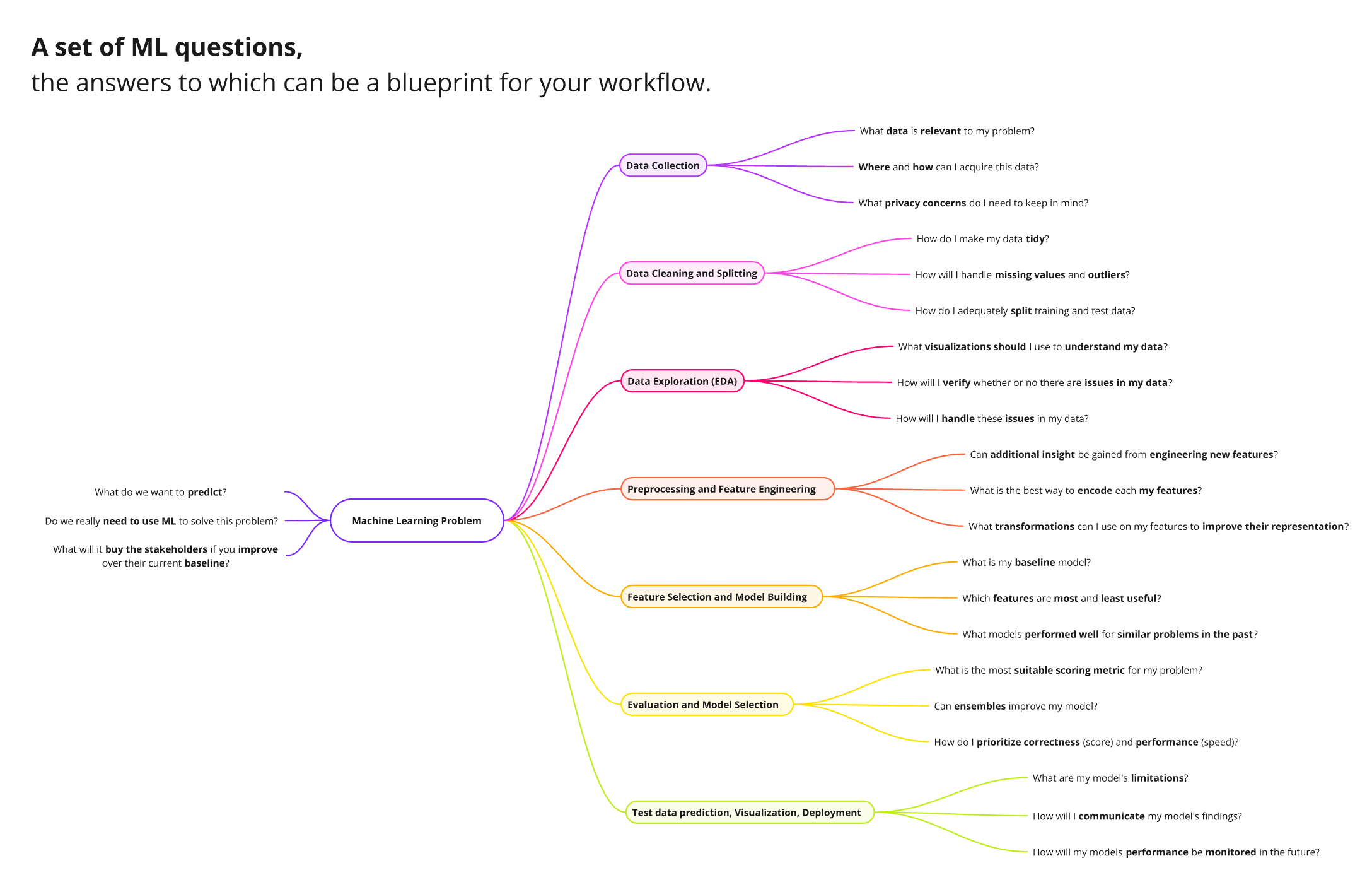 Figure 1: A set of questions to guide you through the ML workflow.
1. Problem Definition
Before diving into data cleaning and modeling, we first have to validate whether ot not our problem is actually an ML problem. Generally, if you answer is yes to the following questions, then you have a ML problem:
- Does the problem require reaching a certain output based on a set of inputs?
- If not, it is unlikely that you will be able to build and train a ML model to achieve the desired result. Keep in mind that this doesn’t necessarily mean you should give up, but rather look for ways to reframe your perspective on the problem to make it more suitable for ML. For example, instead of asking “How can I increase the number of subscribers to my blog”, ask “What features of my blog are most associated with a change in the number of subscribers?”. These “Features” can be any data input you have access to that you believe may impact your result. If your problem is more general rather than personal, you may find the data your looking for in one of the plethora of open data source on the internet (e.g., https://www.kaggle.com/datasets).
- Do we have access to a reliable set of data that will help us reach our goal?
- If not, you may attempt to manually collect the required data yourself (keep in mind that the quality of your results will depend greatly on the quality and size of your data). If you cannot find a way to access or collect the data, then I’m afraid no ML model will be able to help you.
- Is the data so large that a human being cannot effectively read it and use it to solve the problem?
- If not, you are likely better off manually looking for patterns and using simple calculations to reach your goals. As ML models require a large amount of data to be effective.
Congratulations! If you’ve reached this point that means you have already broken down your problem into a set of inputs (features) that influence a particular output (target). And you’ve determined a reliable source of data that will be used to train your model, and you’ve (roughly) determined that your data set is large enough to be used in ML.
2. Preparing our workspace
In this section, we simply want to mindfully prepare a workspace within which we will perform the majority of our analysis work. Although there are many different pieces of software that we can use for this, in this guide we will be using the Pandas package in the Python programming language using VS Code:
- Install Python: https://www.python.org/downloads/
- Python is a programming language that houses numerous packages that contain handy tools that will help us perform our analysis. It is the most popular programming language for ML purposes.
- Install the “conda” package to manage your environments.
- Install VS Code: https://code.visualstudio.com/download
- VS Code is the world’s most popular integrated development environment (IDE).
- I also recommend you install the Jupyter extension within VS Code.
- Create a folder that will store all of your analysis files.
- Create a new conda environment to host the packages you will use for your analysis.
- Install the “pandas” package for data manipulation.
- install the “sklearn” package which contains an assortment of ML models and utilities.
- Install the “matplotlib” package for data visualization. (“altair” is a great option as well).
- Feel free to install any additional packages that you believe will be useful for your analysis.
3. Data Collection
Although we have already determined a source for our data, we still need to transform our data into a tabular structure that makes it easy to feed into an ML model. Here is a list of common data formats and some ways you can transform them into the structure we need:
- Tabular Data (.CSV, .TSV, .XLS, .XLSX, etc.) - No transformation need. You’re good to go into the next part!
- Relational Data (MySQL, PostgreSQL, etc.) - Use SQL connector libraries such as “mysql-connector-python” for MySQL or “psycopg2” for PostgreSQL.
- Non-relational Data (NoSQL, MongoDB, etc.) - Use NoSQL connector libraries such as “pymongo” for MongoDB.
- Media (Images, Videos, Audio) - This type of data is a bit tricky and has to be handled differently. For now it is out of the scope of this guide.
Sample code :
import pandas as pd

raw_data = "data/2023_Property_Tax_Assessment.csv"
housing_df = pd.read_csv(raw_data)
4. Data Cleaning and Splitting
- Ensure your data is tidy:
- Each variable forms a column.
- Each observation forms a row.
- Each type of observational unit forms a table.
- Split your data into training and test sets.
- A generally good split is 80% training data and 20% test data.
- Depending on the size of your data you may need to adjust the split to have more accurate test results.
Sample code :
from sklearn.model_selection import train_test_split

tidy_df = df.melt(id_vars="Name", var_name="Subject", value_name="Score")

# Splitting our tidy data into training and test data
train_df, test_df = train_test_split(tidy_df, test_size=0.3, random_state=123)
5. Data Exploration
- Look at the head and tail of your dataset.
- Look at the types, minimums, maximums, means, and medians of your features. (tip: you can use “describe()” to quickly analyze such metrics).
- Use visualization libraries such as “matplotlib” and “altair” to look at how your data is distributed.
- This will give you an idea of what to expect from your data and you will be able to see any patters or potential issues from the distribution.
Sample code :
import altair as alt

# Create a histogram for assessment values
histogram = alt.Chart(housing_df).mark_bar().encode(
        alt.X("assess_2022:Q", bin=alt.Bin(maxbins=2000), title="Assessment Value").scale(domain=(0, 2000000), clamp=True),
        alt.Y("count():Q", title="Frequency"),
    ).properties(
        title="Distribution of House Assessment Values (2022)"
    )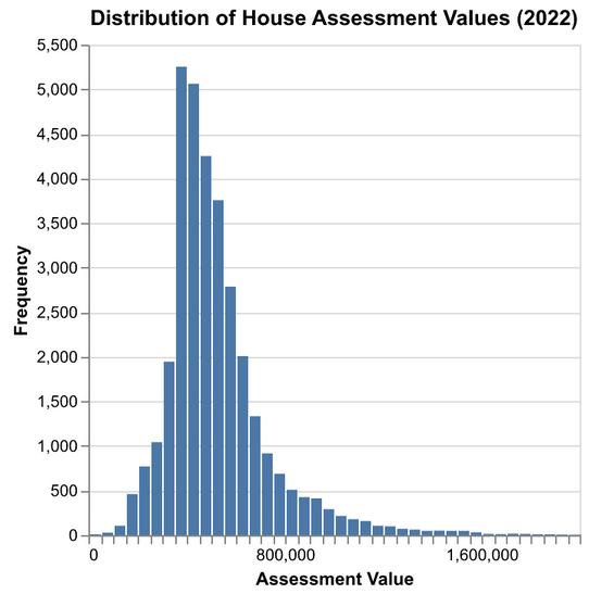
Figure 2: An example of exploratory data analysis using a histogram.
6. Preprocessing and Feature Engineering
- Preprocessing refers to the process of translating a feature into a different scale or form to make it easier for our model to understand it. Here are some basic preprocessing technique that you can use depending on a features data type:
- Numeric features: Standard Scaler.
- Categorical features: One-Hot Encoding.
- Binary features: Represent with 0 and 1.
- Text features: Bag-of-Words if syntax doesn’t matter. NLTK if syntax does matter. (This one is tricky and has many different approaches. The best approach depends on your specific problem).
- Date and time features: Extract meaningful components (e.g., year, month, day, hour, day of week). (This is another tricky one that has plenty of approaches. Depending on your problem and model the best approach may change).
- Keep in mind that there are plenty more types of features and plenty more preprocessing techniques, these examples are only meant to serve as a starting point.
- Feature Engineering can be tricky so feel free to skip this step if this is your first time using ML. Essentially, feature engineering uses existing features and information to create new features that describe the same information from a different angle that can be more beneficial for our model. For example, you may use a “Date of Birth” feature to create a new feature “Age” which can be easier to work with since it is a simple numeric feature rather than a date.
Sample code :
from sklearn.compose import make_column_transformer
from sklearn.preprocessing import OneHotEncoder, StandardScaler

# Divide features by type
categorical_features = ['garage', 'firepl', 'bsmt', 'bdevl']
numeric_features = ['meters']

# Create the column transformer to preprocess features
preprocessor = make_column_transformer(
    (OneHotEncoder(), categorical_features),  # One-hot encode categorical columns
    (StandardScaler(), numeric_features),  # Standardize numeric columns
)
7. Feature Selection and Model Building
- Although we generally like feeding our model as much data as possible, more features doesn’t necessarily result in better performance. In fact, a large number of features can confuse our model and cause “overfitting” which will worsen its performance.
- We have to be selective about which features to keep.
- Start by removing unique features such as IDs, phone number, etc. We want to remove these because they are unlikely to contain any valuable patterns that will benefit our model.
- Remove any other features that you think will have little or no impact on our target
- Don’t worry, you will have the opportunity to come back later and bring back or remove some more features to see how they impact your model.
- Now is a good time to do some research on what ML models generally work well for your type of problem. Here is a short list of well known models and when to use them:
- Linear Regression
- Use for: Predicting a continuous numerical value.
- Example: Predicting house prices based on its size, location, and number of bedrooms.
- Logistic Regression
- Use for: Binary classification problems.
- Example: Predicting whether a customer will churn.
- Decision Trees
- Use for: Interpretable models for classification or regression.
- Example: Classifying loan approvals based on credit scores, income, etc.
- Random Forest
- Use for: Handling complex classification and regression tasks with reduced overfitting.
- Example: Predicting customer segments for marketing campaigns.
- Gradient Boosting (e.g., XGBoost, LightGBM, CatBoost)
- Use for: Complex non-linear relationships and feature interactions.
- Example: Predicting loan default probabilities or rankings.
- Support Vector Machines (SVM)
- Use for: Classification problems, especially with small or high-dimensional datasets.
- Example: Classifying emails as spam or non-spam.
- K-Nearest Neighbors (KNN)
- Use for: Simple classification or regression problems.
- Example: Recommending products based on user similarity.
- Naive Bayes
- Use for: Text classification with large datasets.
- Example: Classifying sentiment in customer reviews.
- Linear Regression
- If you feel indecisive about which one to use, fret not, it is totally valid to find the best model for your problem using trial and error.
- Keep in mind that you can also use an “Ensemble” of a number of these models. But this is a more advanced technique that we will save for another time.
- You also want to create a “dummy” model to act as your baseline to help you gauge your model. Examples include “DummyClassifier” and “DummyRegressor”.
Sample code :
from sklearn.linear_model import RidgeCV
from sklearn.dummy import DummyRegressor
from sklearn.pipeline import make_pipeline

ridge_pipeline = make_pipeline(preprocessor, RidgeCV())
dummy_pipe = make_pipeline(preprocessor, DummyRegressor())
8. Evaluation and Model Selection
- Use cross-validation to evaluate the model you created.
- Go back and redo your feature selection and preprocessing to see how it affects your models performance.
- Try different models and compare them against each other.
- Continuously iterate through this process until you achieve a satisfactory validation score.
Sample code :
from sklearn.model_selection import cross_validate

# initialize results dictionary
cross_val_results = {}

# Perform cross-validation for ridge model
cross_val_results["ridge"] = pd.DataFrame(
    cross_validate(ridge_pipeline, X_train, y_train, return_train_score=True)
).agg(['mean', 'std']).round(3).T

# Perform cross-validation for dummy model
cross_val_results["dummy"] = pd.DataFrame(
    cross_validate(dummy_pipeline, X_train, y_train, return_train_score=True)
).agg(['mean', 'std']).round(3).T
| ridge | dummy | |
|---|---|---|
| fit_time | 0.019 | 0.012 |
| score_time | 0.004 | 0.003 |
| test_score | 0.764 | 0.304 |
| train_score | 0.812 | 0.289 |
Figure 3: Table showing cross validation results of our ridge and dummy models. Please note that “test_score” here actually refers to the validation score and is different from the test score that we will get from our test data later on.
9. Test data and Predictions
- Once you are finally satisfied with your model, test it one last time using the previously unseen “test data”
- Keep in mind that you can only do this once, and you should not go back and adjust your model to try and get a better test score as it will no longer be truly “unseen”. We call this the “golden rule”.
- Congratulations! your model is finally ready to start making predictions.
- These predictions will likely be as accurate as the test score suggests.
- Now all that’s left is to communicate your findings and use those predictions to solve your problem.
Well done! You are now ready to tackle your problems using Machine Learning.
References
- Daumé III, H. (retrieved 2024). A Course in Machine Learning (CIML). Retrieved from https://ciml.info/
- Mueller, A. C., & Guido, S. (2016). Introduction to Machine Learning with Python: A Guide for Data Scientists. O’Reilly Media.
- Russell, S., & Norvig, P. (2020). Artificial Intelligence: A Modern Approach (4th ed.). Pearson.
- Top IDE Index. (retrieved 2025). PYPL Popularity of Programming Languages. Retrieved from https://pypl.github.io/IDE.html